Evidence that curtailing proactive policing can reduce major crime

For benchmarking purposes, each CompStat reports data both for the current year and for the same seven-day range in the previous year. Thus, the 2015 CompStats include 2014 data, and the 2014 CompStats include 2013 data, with weeks matched by their calendar start and end days. The 2014 data contained in the 2014 and 2015 CompStats do not perfectly align, however. Because of when the 52nd week of the previous year finished, week 1 of 2014 begins on 30 December 2013, and week 1 of 2015 begins on 29 December 2014. As a result, the weekly 2014 totals from the 2015 CompStats are off by one day compared with the weekly 2014 totals from the 2014 CompStats. While the choice of how to cut the data does not meaningfully impact our results, we constructed our data set in the following way. Necessarily, 2013 data are taken from the 2014 CompStats, and 2015 data from the 2015 CompStats. But because there are two observations for each week in 2014 (one from the 2014 reports, one from the 2015 reports), we are forced to adopt a rule for which values to use. Because our treatment and control series span multiple years by approximately three weeks in the beginning of January, we reasoned that the best criterion to use to subset the data is to maintain internal consistency within each series. To accomplish this, we used only the 2014 CompStats for all weeks measured as part of the control series, and only the 2015 CompStats for all weeks of the treatment series.

For several reasons, we are confident that the results are not affected by the one-day difference in the series. First, since the ‘Intervention’ is estimated by averaging over a seven-week period, days contained within the five middle weeks overlap completely, leaving only two weeks that are off by a day. Second, we replicated the analyses by averaging the 2014 weeks from the 2014 and 2015 reports. This approach yields comparable results, but because only a single data point is available for each week in 2013 and 2015, we prefer to maintain the data’s internal consistency, rather than introduce another manipulation.

Since our data come from the NYPD, it is worth considering potential sources of bias in police reporting. Concerns have been raised about police data being influenced by the officers tasked with collecting statistics, as well as their superiors25. Still, we feel confident in the CompStat data for several reasons. First, police data are often strongly preferable to alternative sources. Because police records contain a more extensive listing of activity, they are often used to identify the form and extent of bias in other data sources. Second, to minimize the biases associated with human error, the NYPD requires officers to apply a ‘strict interpretation bias’. When reporting a crime complaint, an officer must enter the incident on the basis of the most serious crime described by the claimant, regardless of whether the officer believes the perpetrator can be tried or arrested for that offence. This procedure was put into place under the theory that strict interpretation bias would increase the willingness of individuals to come forward with crime complaints. As a result, the majority of errors in the categorization of a crime should lead to upgrading, rather than downgrading, the criminal classification25.

Any remaining bias from manipulation by police officers would predispose the study towards identifying an escalation in major crime complaints. Prior to the slowdown, precinct commanders’ interest lay in demonstrating continuing declines in crime. Professional incentives reversed during and after the slowdown insofar as commanders wished to demonstrate the necessity of the police force and the effectiveness of their policing strategies.

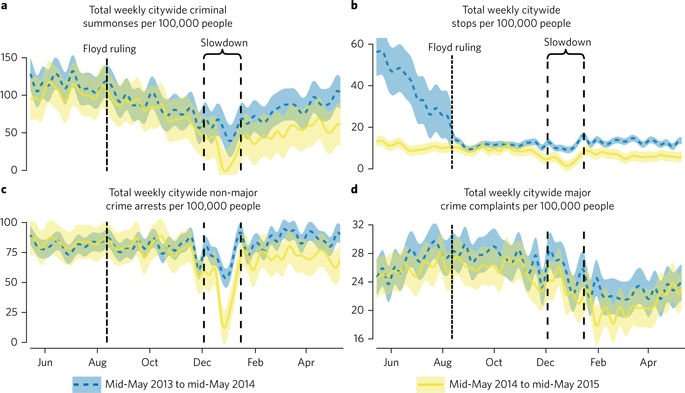
With regards to police protocol, there were three important changes in NYPD procedure during our time series worthy of mention. First, on 31 October 2013, an appellate court ruled on ‘Floyd versus City of New York’, ordering NYC to eliminate racial profiling in the NYPD’s stop-and-frisk encounters. We display the corresponding sharp decline in these encounters in Fig. 1. Our analyses control for the effects of the ‘Floyd’ decision by including precinct-week counts of SQFs in models of other police and criminal behaviours, and a dummy for the pre- and post-‘Floyd’ periods in model (2) of Fig. 2, as SQFs are the outcome. Second, in July 2014, the Brooklyn District Attorney Ken Thompson declared that his office would no longer prosecute marijuana possession under certain conditions. Third, on 19 November 2014, NYC formally decriminalized marijuana possession, making it a summons rather than an arrestable offence. While these three procedural changes surely impacted policing practices, their causes are unrelated to the slowdown, and thus we should not expect them to impact our causal estimation. Indeed, our analyses in Fig. 4 and Supplementary Fig. 8 show that the timing of changing patterns of compliance corresponds to the period of the slowdown, rather than these earlier procedural changes.

With regards to data availability, we encountered missingness in two situations. The first concerns three of our measures of police strength and strategy. The number of officers per precinct is from 2007, and the number of Civilian Complaint Review Board (CCRB) complaints is from 2013, and thus predate the formation of the 121st precinct, which became fully operational in July 2013. To address this, we imputed values for this precinct using data from the 120th and 122nd precincts, which were split to form the 121st. We weight these variables’ covariates for all three precincts proportionately on the basis of geographic, and when appropriate temporal, coverage. We did the same for SQFs before July 2013.

The second site of missing data results from the fact that the NYPD has thus far failed to turn over CompStat reports from two weeks in January 2016. In spite of the NYPD’s recalcitrance, we have no reason to suspect that the missing weeks (weeks 2–3 of 2016) impact the results. To empirically demonstrate that our results are not affected by missing data, we take a conservative approach when imputing data for the missing values. In the final column of Fig. 4, we fill in the missing 2016 data with the two weeks from the actual slowdown (in January 2015). We believe this is a better modelling strategy than multiple imputation, which can introduce bias when applied to nonlinear models32. Imputing the missing data using the actual slowdown values also presents a harder test for demonstrating nonsignificance in the placebo treatment as compared with the last observation carried forward. In the first four weeks of the slowdown, rates of major crime complaints were nearly 20% lower as compared with the same period the following year. Replicating the 2015 placebo tests without the imputed weeks produces comparable non-significant results (Supplementary Fig. 5 model (5)).

The systematic component of our econometric model is represented in equation (1). The DiD model estimates changes in police behaviour or civilian crime complaints (Y) as a function of dichotomous indicators of the ‘Series’ (S) and ‘Treatment window’ (T), an interaction of the two (‘Series’ × ‘Treatment window’) representing the ‘Intervention’ period (STT = I), and a variety of covariates (X)33,34.

A critical requirement of the DiD modelling strategy is the ‘parallel trends’ assumption. To reliably estimate differences during the treatment window, the data must follow the same pattern outside the window. Figure 1 confirms that the control series indeed provides a reliable baseline from which to measure any changes induced by the slowdown.

We estimate the models using a negative binomial specification (Y i ≈ NegBin(r i , p)) because all outcome variables are overdispersed count data, as revealed by two types of dispersion test. For the base model using ‘Major crime complaints’ as the outcome variable (Fig. 3 model (1)), a likelihood ratio test of the null hypothesis that the Poisson model restriction of equal mean and variance is true is rejected with a χ2(1) value of 2,377 (P< 0.001, two-sided). Results are comparable for all other models (see Supplementary Tables 1–3). Ordinary least squares is even less appropriate than Poisson, as the dependent variables are neither normally distributed nor interval. Furthermore, because observations within precincts are not independent, and hence their errors are correlated, we calculate robust standard errors clustered by precinct.

While the slowdown in policing is arguably independent from precinct-level covariates, we include a number of controls in case these variables influence the precincts’ responsiveness to the slowdown. Including controls such as population and other demographic characteristics helps to normalize the variance in the dependent variables across precincts. Because it lacks a residential population, all analyses exclude the Central Park Precinct. We use the most recent demographic data, which are taken from the 2014 five-year American Community Survey (ACS). Using the ACS, we identified each precinct’s ‘Population’, as well as the crime-prone age group ‘Percentage aged 15–24’.

We also include a number of key indicators of concentrated disadvantage. Using data from the ACS, we generated precinct-level measures of ‘Average family income’, ‘Percentage of residents who are persons of colour’, ‘Percentage unemployed’ and several household-level measures, including ‘Percentage of households on public assistance’, ‘Percentage of households headed by women with children’, ‘Percentage of occupied housing units rented’ and ‘Percentage of households vacant’. Because these factors loaded poorly on a single dimension as well as on two dimensions, all analyses with covariates incorporate these variables individually (see Supplementary Tables 1–3). In Supplementary Fig. 5 model (3), we report a replication using our measure of concentrated disadvantage, which is defined as the mean of the standardized (that is, centred at 0 and scaled such that standard deviations are equal to 1) values of ‘Percentage of residents who are persons of colour’, ‘Percentage unemployed’, ‘Percentage of households on public assistance’ and ‘Percentage of households headed by single women with children’. The model accordingly does not include these constituent variables individually to avoid collinearity.

Our models also control for precinct-level variation in policing capacity and behaviour. In addition to the total precinct-week SQFs mentioned earlier, we construct per capita precinct-level variables of the number of officers assigned to a precinct in 2007 (‘Officers per 100,000 people’) and complaints registered against the precinct with the CCRB in 2013 (‘CCRB complaints per 100,000 people’) using data from previous research35. The CCRB data also provide an indicator of the distribution of complaints across racial groups, which we measure as ‘Percentage of CCRB complaints by persons of colour/percentage of residents who are persons of colour’.

We further include three weather-related controls, each of which are weekly averages of daily measures for NYC from the National Weather Service: ‘Mean temperature’, ‘Total rain accumulation’ and ‘Total snow/sleet accumulation’. To account for temporal autocorrelation and geographic spillover effects, all models include a one-week ‘Spatial lag’ of the dependent variable. To construct this, we identified adjacent, contiguous precincts for each precinct, and calculated the mean of the previous week’s values. Because NYC is composed of multiple islands connected by bridges and tunnels, we deem this more appropriate than using an inverse distance weighted measure. The choice does not meaningfully alter the results.

Lastly, while Fig. 1 lends support to the parallel trends assumption necessary to DiD, we include two additional controls for temporal variance in policing and criminal behaviour. First, to adjust for the ongoing downward trend in crime, we include a ‘Time counter’, which counts the number of weeks since the first week of the time series, starting at 1. Second, alongside the three weather-related variables, we include dummy variables for ‘Summer’, ‘Autumn’ and ‘Winter’ to help control for seasonal effects.

Using our fitted model, we estimate our causal effects as shown in equation (2), where τ ̄ represents the average treatment effect on the treated (ATT):

Y 1 and Y 0 represent potential outcomes had the ‘treatment’ (e.g., the slowdown in Figs. 2 and 3) occurred versus had it not. N τ is the number of observations in the intervention period, which are index by i. The percentage change in the outcome induced by the ‘Intervention’ is:

100 × τ ̄ ∑ i = 1 N τ exp α ^ + γ ^ + λ ^ + X i β ^ The standard error can be found by applying the delta method to the exponentiated coefficient, multiplied by the average predicted counterfactual. Significance is assessed with z-tests.

In words, our procedure for calculating causal effects is as follows. We generate ATTs by averaging the precinct-week differences between the predicted value with the ‘Intervention’ set to 1 versus set to 0 during the ‘Intervention’ period (that is, the average difference between the values predicted for each precinct-week observation had the slowdown occurred versus had it not, all else equal)33. The ATT is converted to an average predicted weekly percentage change by dividing it by the mean predicted counterfactual and multiplying by 100. Figures 2–4 graphically present the average predicted percentage change and corresponding 95% confidence intervals with delta method standard errors clustered by precinct, as well as report the raw ATTs and their standard errors and P values. Statistical significance is determined using two-tailed z-tests. More detailed results for the models in Figs. 2–4 can be found in Supplementary Tables 1–3.

While we believe that DiD is the best modelling approach given our data and the nature of criminality and policing, we also ran ITS models using the entire time series. In the ITS analyses, we replicate the modelling approach adopted in earlier research on police slowdowns, with the addition of our precinct-level control variables30. Results from the base specification comparing ITS with the DiD estimates are presented in Fig. 3. Results from a full replication of all models using ITS instead are displayed in Supplementary Figs. 2–4. We contend, however, that DiD is more appropriate primarily for three reasons. First, with ITS, the modeller must specify the functional form of the proposed trends before, during and after the ‘treatment’. The most common assumption is that trends are linear. In Fig. 3 we do not include such additional trend shifts for simplicity, but doing so does not alter the results. In Supplementary Fig. 7 we show that the predicted values from a specification in which we include slowdown and post-slowdown trend shifts results in counterfactual predictions during the slowdown that closely mirror those of the base DiD model from Fig. 3 model (1). Second, ITS is especially sensitive to seasonal effects, and while there are different ways to control for them, none are perfect. Third, and most importantly, the treatment window overlaps very closely with (meteorological and astronomical) winter, exacerbating the previously mentioned issue, especially because it is a time of depressed crime in general. DiD does not require imposing as much structure, and controls for cyclical trends by design. Regardless, the ITS results are essentially the same.

Lastly, while interaction terms in nonlinear models are not usually equal to the product term, in the special case of difference-in-differences models, identification of the ATT is as simple as equation (2)33,34. The same holds for ITS models that do not include trend shift variables. In such cases, the ATT is similarly derived from the level shift coefficient. Adding trend shift variables, however, introduces considerable complexity for two reasons: first, they are products of interacting level shifts with the time trend; and second, the total treatment effect is the combination of the multiple effects. While the point estimate of the ATT can be calculated using the average predicted change during the intervention period, standard errors are not as easily obtained. We ran such models and found that the ATTs and ‘Intervention’ level shift coefficients and standard errors were nearly identical to models without the trend shifts. Therefore, we focus on the simpler case in Fig. 3 model (3) and Supplementary Figs. 2–4.

The computer code that support the findings of this study is available from the corresponding author upon reasonable request.

The data that supports the findings of this study are available from the corresponding author upon reasonable request.