Calculation of external climate costs for food highlights inadequate pricing of animal products

In this section, first, we outline the method as a whole to give the reader an orientation and context for the following two parts. Second, we discuss the input data (for quantification and monetization). Third, we explain the merging of all input data, and thus the calculation of the output data. Finally, we address the influence of uncertainties on our method. The reference year for this analysis is 2016, and the reference country is Germany, which is listed as the third most affected country in the Global Climate Risk Index 2020 Ranking70.

We differentiate between two steps within this method of calculating food-category-specific externalities and the resulting external costs. These are first the quantification and second the monetization of externalities from GHGs (visualized in Fig. 3). We use this bottom-up approach following the example of Grinsven et al.10, who conducted a cost-benefit analysis of reactive nitrogen emissions from the agricultural sector. This two-stepped method also allows the adequately differentiated assessment for GHG emissions of various food categories.

Fig. 3: Visualization of the method. The method includes quantifying and monetizing product-specific externalities. In the case of Germany, emission data were obtained from the Global Emission Model for Integrated Systems (GEMIS)44. We used production data from the German Federal Statistical Office88 and AMI89,90, and calculated the emission difference between organic and conventional production based on a meta-analytical approach (see “Results” subsection on input data for quantification). The category-specific emission data were calculated on the basis of these input data. The emission cost rate was obtained from the German Federal Environmental Agency (UBA)32. The category-specific external costs were determined on the basis of the previously developed price-quantity-framework (see “Results” subsection on input data for monetization). Full size image

The quantification includes the determination of food-specific GHG emissions—also known as carbon footprints39—occurring from cradle to farmgate by the usage of a material-flow analysis tool. Carbon footprints are understood within this paper in line with Pandey et al.71 where all climate-relevant gases, which (in addition to CO 2 ) include methane (CH 4 ) and nitrous oxide (N 2 O), are considered. Their 100-year CO 2 equivalents conversion factors are henceforth defined as 28 and 265, respectively72. Here, the material-flow analysis tool GEMIS (Global Emission model for Integrated Systems)44 is used, which offers data for a variety of conventionally farmed foodstuff. As GEMIS data focus on emissions from conventional agricultural systems, we carried out the distinction to organic systems ourselves. We determined the difference in GHG emissions between the systems by applying meta-analytical methods to studies comparing the systems’ GHG emissions directly to one another. Meta-analysis is commonly used in the agricultural context, for example, when comparing the productivity of both systems57,58,59 or their performance1.

For better communicability, we first aggregate the 11 food-specific datasets given in GEMIS to the broader food categories plant-based, animal-based, and dairy by weighting them with their German production quantities (cf. “Results“ subsection on quantification). On top of that, LUC emissions are calculated for conventional foodstuff.

Through monetization, these emission data are translated into monetary values, which constitute the category-specific external costs. The ratio of external costs to the foodstuff’s producer price represents the percentage which would have to be added on top of the current food price to internalize externalities from GHGs and depict the true value of the examined foodstuff.

Starting with the data on food-specific emissions, GEMIS is used because of its large database of life-cycle data on agricultural products with a geographic focus on Germany. GEMIS is a World-Bank acknowledged tool for their platform on climate-smart planning and drew on 671 references, which are traced back to 13 different databases. The German Federal Environmental Agency uses GEMIS as a database for their projects and reports establishing it to be an adequate tool for the German context especially73,74. This tool is provided by the International Institute for Sustainability Analysis and Strategy (IINAS). GEMIS offers a complete view on the life cycle of a product, from primary energy and resource extraction to the construction and usage of facilities and transport systems. As GEMIS only offers data for the year 2010, we conducted a linear regression on the basis of the prevailing emission trend for the German agricultural context in order to align the data with the reference year 201675. For this, annual German emission data from 2000 to 2015 from the Federal Environmental Agency of Germany was used76. On every level of the process chain, data on energy- and material-input, as well as data on output of waste material and emissions, are provided by GEMIS. These data consist partly of self-compiled data from IINAS and partly of data from third-party academic research or other life-cycle assessment tools. Specific information on the data sources is available for every dataset of a product. In this study, the system boundaries for assessing food-specific GHG emissions span from cradle to farmgate. This means that we consider all resource inputs and outputs during production up to the point of selling by the primary producer (farmgate). This includes emissions from all production-relevant transports as well as emissions linked to the preliminary building of production-relevant infrastructure.

We specify that for animal-based products, emissions from feed production, as a necessary resource input, are assigned to these animal-based products. Such emissions naturally should include LUC emissions. LUC emissions are of negligible proportion for locally grown products, as agricultural land area is slightly decreasing in Germany47. Thus, we have to focus solely on imported feed for conventional animal-based and dairy products. Organic feed is not considered as article 14d of the EU-Eco regulation stipulates that organic farms have to primarily use feed which they produce themselves or which was produced from other organic farms in the same region77. The region is understood as the same or the directly neighboring federal state46. Although the EU-Eco regulation does not completely rule out fodder imports from foreign countries, it limits its application significantly. Also, one has to consider that over 60% of the organic agricultural area belongs to organic farming associations78. These associations stipulate even stricter rules than the standard EU-eco regulation. Examples are Bioland, where imports from other EU and third countries are only allowed as a time-limited exception79, Naturland, where additionally imports of soy are banned completely80, or Neuland, that ban any fodder imports from overseas81. We thus assume that the emissions that could possibly be caused by organic farming in Germany through the import of feed constitute a negligibly small fraction of the total emissions of a product. Thus, we follow common assumptions from the literature82,83,84 and calculate no LUC emissions for organic products. For conventional products, we calculate LUC emissions by application of the method of Ponsioen and Blonk45. This method allows the calculation of LUC emissions for a specific crop in a specific country for a specific year. With regards to the year, we apply our reference year 2016. With regards to crop and country one has to keep in mind that in the case of Germany, the net imports of feed are the highest for soymeal, followed by maize and rapeseed meal, making up over 90% of all net positive feed imports85. Maize and rapeseed meal are both imported mainly from Russia and Ukraine (93% and 87% of all imports86). Taken together, the crop area of Russia and Ukraine is decreasing by 150,000 ha/year (data from 1990 to 2015 were used87). Following Ponsioen and Blonk45, we thus assume that there are no LUC emissions of agricultural products from these countries. This leaves us with soymeal, of which 97% are imported from Argentina and Brazil. We thus calculate LUC emissions of soymeal for Argentina and Brazil, respectively. Data are used from Ponsioen and Blonk45, except for the data of the crop area, where updated data from FAOSTAT are used in order to match the reference year. We then weigh those country-specific emission values according to their import quantity. This results in 2.54 kg CO 2 eq/kg soymeal. To incorporate this value into the conventional emission data from GEMIS, we map the LUC emissions to all the soymeal inputs connected to the food-specific products.

For aggregation to narrow categories, we categorize every dataset from GEMIS into one of the eleven narrow food categories. The choice of separation into these specific categories is based on the categorization of the German Federal Office of Statistics88 from which production data were obtained. According to one category’s yearly production quantity, we incorporate every food product into the weighted mean of its corresponding food category. Thus, the higher a food’s production quantity, the greater the weight of this product’s emission data in the broad category’s emission mean. All data on the production quantities refer to food produced in Germany in the year 2016. For this weighting and aggregation step, only production quantities used for human nutrition were considered, thus feed and industry usage of food are ruled out (in contrast to emission calculation, where feed is indeed considered). Besides the German Federal Office of Statistics88, the source for this data is the German Society for Information on the Agricultural Market (AMI)89,90. Only production data for conventional production is used. Thereby, we imply ratios of production quantities across the food categories for organic production that are equal to those of conventional production. This does not fully reflect the current situation of organic production properties but allows for a fair comparison between the emission data of organic and conventional food categories. Doing otherwise would create ratios between emission values of organic and conventional broad categories that would not be representative of the ratios between organic and conventional narrow categories. In Table 4, all production data are listed, whereby total production quantities in 1000 t can be found in the right column. Translating these into percentage shares, the column right to the narrow category’s column represents the shares of the specific foods inside the narrow categories, whereas the column right to the broad category’s column represents the shares of the narrow categories inside the broad categories. These shares are expressed in formula 2a and 2b (see “Method and data” subsection on output data) by the terms \(\frac{{p_{b,n,conv}}}{{P_{b,conv}}}\) (share in broad categories) and \(\frac{{q_{b,n,i,conv}}}{{p_{b,n,conv}}}\) (share in narrow categories).

We aggregate GEMIS emission data (q b,n,i,conv ) to narrow (e b,n,conv ) and broad categories (E b,conv ) by multiplying the respective emission data with the shares from Table 3 (cf. formula 2a and b, “Method and data“ subsection on output data). From these conventional emission values, we derive emissions for organic production. For narrow as well as broad categories, the respective conventional emission values are multiplied with the applicable emission differences D b,org/conv (cf. Table 2).

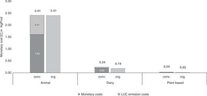
With these data, we aggregate the above mentioned eleven food categories to three broad categories: plant-based, animal-based, and dairy. Besides the obvious differentiation between animal- and plant-based products, dairy is considered separately from other animal-based products because of its relatively high production volume and its, in contrast to that, relatively low externalities. Because the weighted mean of the three main categories is affected by the production quantities of its corresponding subcategories, mapping dairy into the animal-based category would otherwise distort the emission data of this very category.

As outlined before, only data regarding externalities of conventional agricultural production are included in GEMIS and could therefore be aggregated. Nevertheless, by applying meta-analytical methods regarding the percentage difference of GHG emissions between conventional and organic production, we derive the emission data for organic production for each of the broad categories (plant-based, animal-based, and dairy). It has to be noted that LUC emissions are consistently excluded at this level of calculation. To derive emission differences between organic and conventional farming, research was conducted by snowball sampling from already existing and thematically fitting meta-analysis, by keyword searching in research databases, as well as forward and backward search on the basis of already-known sources. Criteria for selected studies were climatic and regulative comparability to Germany. In the selected studies, relative externalities between conventional and organic farming are compared in relation to the cropland. To cover a reasonably relevant period, we decided to search for studies published within the past 50 years (from 1969 to 2018) and could therefore identify fifteen relevant studies, spanning from 1995 to 2015. Four of these studies have Germany as their reference country while the other eleven focus on other European countries (Denmark, France, Ireland, Netherlands, Spain, UK; please consult Table 2 for specifics). The weighted mean of the individual study results amounts to the difference in GHG emissions between the two farming production systems. As the selected studies are based on geophysical measurements and not on inferential statistics, a weighting based on the standard error of the primary study results like in standard meta-analysis91 was not possible. We aimed for a system that weights the underlying studies regarding their quality and therefore including their results weighted accordingly in our calculations. Within the scope of classic meta-analyses92, the studies’ individual quality is estimated according to their reported standard error (SE), which is understood as a measure of uncertainty: the smaller the SE, the higher the weight that is assigned to the regarding the source. Due to the varying estimation methods of considered studies, the majority of considered papers does not report measures of deviation for their results. These state definite values; therefore, there is no information about the precision of the results at hand. Against this background, we have decided to use a modified approach to estimate the considered papers’ qualities93. Following van Ewijk et al.94 and Haase et al.95, we apply three relevant context-sensitive variables to approximate the standard error of the dependent variable and thereby evaluate the quality of each publication: the newer the paper (compared to the timeframe between 1995 and 2018), the higher we assume the quality of reported results. The more often a paper was cited per year (measured on the basis of Google Scholar), the higher the paper’s reputation. The higher the publishing journal’s impact factor (measured with the SciMago journal ranking), the higher its reputation and therefore, the paper’s quality. For every paper, the three indicators publishing year (shortened with PY in Table 2), citations/year (CY), and journal rank (SJR) rank a paper’s impact on a scale from 1 to 10, where 1 describes the lowest qualitative rank and 10 the highest. The sum of these three factors (SUM) then determines the weight of a paper’s result in the mean value (WEIGHT). The papers’ reported emission differences between organic and conventional (diff. org/conv) are weighted with the papers’ specifically calculated WEIGHTS and finally aggregated to the emission difference between both systems.

With this approach, we weight results of qualitatively valuable papers higher and are therefore able to reduce the level of uncertainty in the estimated values because standard errors could—due to inconsistencies in the underlying studies—not be used. The results of this meta-analytical approach are listed in Table 2 (cf. “Results” subsection on quantification); further details can be found in Supplementary Note 1 and Supplementary Table 1. The studies considered compare GHG emissions of farming systems in relation to the crop/farm area. However, since our study aims to compare GHG emissions in relation to the weight of foodstuff, we include the difference in yield (yield gap) between the two farming systems for plant-based products and the difference in productivity (productivity gap) for animal-based and dairy products. For plant-based products, the yield gap is 117%, meaning that conventional farming produces 17% more plant-based products than organic farming in a given area. This gap was derived from three comprehensive meta studies57,58,59 and weighted as just described for the emission difference between organic and conventional farming. For animal-based as well as dairy products, the productivity gap could be determined with the same studies used for the meta-analytical estimation of the emission differences22,23,24,25,28,95. The productivity gap is 179% for animal-based and 152% for dairy products. In line with Sanders and Hess63, the yield (or productivity) difference \(\frac{{yield_{conv}}}{{yield_{org}}}\) affects the calculation of the food-weight-specific emission difference \(\frac{{GHG_{org\;food\;weight}}}{{GHG_{conv\;food\;weight}}} = D_{org/conv}\) between both farming systems: the yield difference is hereby multiplied with the cropland-specific emission difference \(\frac{{GHG_{org\;cropland}}}{{GHG_{conv\;crioland}}}\). Resulting from this, the emission difference can be formulated as follows:

$$D_{org/conv} = \frac{{GHG_{org\;food\;weight}}}{{GHG_{conv\;food\;weight}}} = \frac{{GHG_{org\;cropland}}}{{GHG_{conv\;cropland}}} \times \frac{{yield_{conv}}}{{yield_{org}}}$$ (1)

If the yield difference were not included, emissions from organic farming would appear lower than they actually are as organic farming has lower emissions per kg of foodstuff but also lower yields per area. With formula 1, we adjust for that.

Monetization of these externalities requires data on GHG costs as well as data on the food categories’ producer prices.

The cost rate for CO 2 equivalents used in this study stems from the guidelines of the German Federal Environment Agency (UBA) on estimating external ecological costs32. They recommend a cost rate of 180 € per ton of CO 2 equivalents. This value is very close to the value of the 5th IPCC Assessment Report (173.5 €/tCO 2 eq), where the mean of all (up to this point) available studies with a time preference rate of 1% was determined33. The cost rate from the German Federal Environment Agency’s guideline is based on the cost damage model FUND96 and includes an equity weighting as well as a time preference rate of 1% for future damages. In this model, different impact categories are considered in order to estimate external costs from GHG emissions. Damage costs can be differentiated as benefit losses such as lowered life expectancy or agricultural yield losses and costs of damage reduction such as medical treatment costs or water purification costs97. Following UBA, these damage costs are analyzed in the following categories: agriculture, forestry, sea-level rise, cardiovascular and respiratory disorders related to cold and heat stress, malaria, dengue fever, schistosomiasis, diarrhea, energy consumption, water resources, and unmanaged ecosystems96. Using a cost-benefit-analysis (CBA), an adequate level of emissions is reached when marginal abatement costs are equal with damage costs. In a CBA external damage, costs can therefore be conceptualized as a price surcharge necessary to effect their optimal reduction98.

For the pricing of the food categories, we determine the total amount of proceeds that farmers accumulate for their sold foodstuff in €99 for each category (producer price) divided by its total production quantity. Thereby we calculate the relative price per ton for each foodstuff. We solely refer to producer prices as the system boundaries only reach until the farmgate.

Output data include the aggregation and separation of food-specific categories to the broader categories of animal- and plant-based products, as well as conventional and organic products. As previously explained, such aggregation and separation are needed because the underlying material-flow analysis tool only lists food-specific emission data for conventionally produced foodstuff. Combining the input data, we are now able to quantify and monetize externalities of GHGs for different food categories.

For quantification, we separate between the following two steps: first, the aggregation of emissions data to broader categories and second the differentiation between conventional and organic farming systems. We iterate these steps two times, once for broad categories of animal-based products, plant-based products, and dairy and once for more narrow categories of vegetables, fruits, root crops, legumes, cereal, and oilseeds on the plant-based side as well as milk, eggs, poultry, ruminant, and pig on the animal-based side. Figure 4 displays the whole process of quantification schematically before we describe it in detail in the following text.

Fig. 4: Visualization of the quantification process. Quantification as well as corresponding input and output data are displayed. Data from the Global Emissions Model for Integrated Systems (GEMIS)44 (g b,n,i,conv ) and production data88,89,90 (q b,n,i,conv ) are combined, and emission data for broad (E b,conv ) and narrow (e b,n,conv ) categories are derived for conventional production. Organic emission values are calculated by multiplication of conventional emission values (E b,org and eb,n,org ) with the emission difference (D b,org/conv ) (cf. “Input data for quantification”). Full size image

Concerning the reasoning behind the method, the question that might come to mind is why the differentiation between farming systems happens after the aggregation and not before. This is due to the fact that the proportional production quantities of specific food as well as food categories to each other differ from conventional to organic production. Let us imagine aggregation would take place after the differentiation of farming systems: for example, beef actually makes up over 50% of all produced food in the organic animal-based product category, while it only accounts for 25% of the conventional animal-based product category (cf. production values in Table 3). As beef production produces the highest emissions of all foodstuffs, these high emissions would be weighted far stronger in the organic category than in the conventional category and thereby producing a higher mean for the organic animal-based product category than for the conventional one. As can be seen from this example, the organic animal-based product category could have a higher mean of emissions than the conventional animal-based product category while still having lower emissions for each individual organic animal-based product than conventional production. Deriving GHG emissions of foodstuff before aggregating to broader categories would thus be problematic and create means not representative for the elements that make up the broader category. To prevent this problem, the chosen method in this paper is thus to first aggregate to the chosen level of granularity (broad or narrow food categories) and then to derive emissions of organic production from conventional production data.

The first step of aggregation consists first of aggregating food-specific emission data from GEMIS g b,n,i,conv to the narrow categories e b,n,conv and second aggregating emission data from the narrow categories to the broad categories E b,conv . As mentioned before and remarked in the respective indices, all these data only refer to conventional production up to this point. For both steps, the method is identical. The aggregation to narrow categories is represented in (2a) where e b,n,conv stands for the emissions of the narrow category n, which itself is part of the broad category b. Input data from GEMIS are remarked as g b,n,i,conv , whereby the index i refers to the ith element of category n. It’s production quantity is q b,n,i,conv . p b,n,conv represents the production quantity of the narrow category n. I (and N in formula 2b) represents the highest index of an element in a narrow (or a broad) category.

$$e_{b,n = x,conv} = \mathop {\sum }\limits_{i \in n = x}^I g_{b,n,i,conv} \times \frac{{q_{b,n,i,conv}}}{{p_{b,n,conv}}}$$ (2a)

The aggregation to broad categories is described by formula 2b whereby E b,conv are the emissions and P b,conv the production quantity of broad category b.

$$E_{b = x,conv} = \mathop {\sum }\limits_{n \in b = x}^N e_{b,n,conv} \times \frac{{p_{b,n,conv}}}{{P_{b,conv}}}.$$ (2b)

In the second step, we calculate emission values for organic production by multiplying the calculated emission difference D b,org/conv between both farming systems (cf. “Input data for quantification”) with the conventional emission values. These organic emission values are denoted as E b,org for broad categories and e b,n,org for narrow categories.

To calculate the costs C b of category-specific emissions, we multiply the cost rate P for CO 2 equivalents with the category-specific emission data E b or e b,n (depending on whether broad or narrow categories are observed). Further, we determine percentage surcharge costs \(\Delta _b\) by setting these costs in relation to the producer price pp b of the respective food category: \(\Delta _b = \frac{{C_b}}{{pp_b}}\) (the calculation is analogue for narrow categories). These surcharge costs represent the price increase necessary to internalize all externalities from GHG emissions for a specific food category.

Due to the interdisciplinarity and novelty of our study, we connect several methodological approaches and refer to various sources for data. Against this background, we had to accept some uncertainties while assembling and using the developed framework for our calculation. The studies included in our meta-analytical approach of calculating the difference between organic and conventional emission values, for one, are not fully consistent in the methodologies each of them uses (refer to Supplementary Table 1 for details). Furthermore, from the results of all included studies, it is apparent that there exists a wide range of emission differences between the farming practices, depending on the paper’s scope and examined produce21. We attempted to account for this by performing the studies according to their fit regarding the object of research (cf. “Input data for quantification”). Due to insufficient availability of the data for the emission differences between organic and conventional on the basis of each narrow category, an average for the emission difference was used. This possibly results in imprecisions during the internalization of the external costs on the level of all narrow categories. Therefore, we focus on the aggregated broad categories, as this uncertainty can be evaded here. Furthermore, the in literature reported price factor for CO 2 equivalents is volatile over time, impacting the results of this paper. It is to be expected that the external costs of GHG emissions are likely to rise in the future (cf. subsection on research aim and literature review). Also, our study’s scope is confined to the assessment of the current production situation within the German agricultural sector. Therefore, we do not account for future developments regarding a changing agricultural production landscape after internalization of the accounted external costs. We do, however, discuss possible effects on demand patterns as well as the environmental and social performance of the agricultural sector in “Discussion”. Regarding the incorporated LUC emissions, there appears to be a lacking scientific consensus on a general method of calculation for such emissions45,100,101,102. We thus want to emphasize that these additional emissions should be treated with caution and are thereby displayed separately from the other data.

Further information on research design is available in the Nature Research Reporting Summary linked to this article.